Visualizing Logic: Mastering Karnaugh Maps for Efficient Digital Design

Denny

January 13, 2026 8 min read

Karnaugh map visualization next to a simplified digital circuit, demonstrating logic simplification. — Karnaugh maps provide a visual pathway from complex Boolean equations to elegant, optimized digital circuits, as demonstrated here with a 4-variable example leading to an XNOR gate.

Algebraic simplification using Boolean laws works, but it depends on spotting the right factoring at the right time. Miss one opportunity and you end up with a suboptimal result. For expressions with four or more variables, the number of possible manipulations explodes.

The Karnaugh map (K-map) solves this problem by converting algebraic simplification into visual pattern recognition. Developed by Bell Labs physicist Maurice Karnaugh in 1953, it arranges a truth table into a two-dimensional grid where adjacent cells differ by exactly one variable. Grouping adjacent 1s on the grid directly produces minimal Sum-of-Products expressions — no algebraic manipulation required.

AND Gate Component Diagram

The Visual Truth Table: What is a K-Map?

At its core, a Karnaugh map is a truth table in disguise. While a truth table lists inputs and outputs in a linear, vertical fashion, the K-map rearranges them into a two-dimensional grid. This isn’t just for show. The genius of the K-map lies in its specific arrangement of cells.

In a standard truth table, the rows follow a binary count (00, 01, 10, 11). In a K-map, the rows and columns follow a sequence known as Gray code. In a Gray code sequence, each adjacent number—whether you move horizontally or vertically—differs by only a single bit. This property, known as logical adjacency, is the engine that drives simplification. When you group adjacent cells containing ‘1’s, you are visually identifying variables that change (and thus don’t affect the outcome) and eliminating them, leaving behind a minimal Boolean term.

Before we dive into the complex 4-variable maps used in modern ALU design, let’s look at the fundamental 2-variable map for inputs $A$ and $B$ . It consists of $2^2 = 4$ cells, representing the four possible minterms.

	$B=0$ ( $\overline{B}$ )	$B=1$ ( $B$ )
$A=0$ ( $\overline{A}$ )	$m_0$ ( $\overline{A}\overline{B}$ )	$m_1$ ( $\overline{A}B$ )
$A=1$ ( $A$ )	$m_2$ ( $A\overline{B}$ )	$m_3$ ( $AB$ )

Notice the adjacency: moving from $m_0$ to $m_1$ , only variable $B$ changes. Moving from $m_1$ to $m_3$ , only variable $A$ changes. This physical proximity on the grid represents a logical relationship that we can exploit to reduce our gate count.

See Basic Logic in Action

The Art of Grouping: From Maps to Minimal Logic

The goal of using a K-map is to cover all the ‘1’s in the map using the largest possible rectangular groups. However, there’s a catch: the number of cells in each group must be a power of two (1, 2, 4, 8, 16, and so on). Each group you draw corresponds to a simplified product term. Your final, optimized expression is simply the “Sum of Products” (ORing the results of those groups).

The grouping rules are strict but straightforward. Following them mechanically guarantees a minimal result.

Cover Every ‘1’: Every ‘1’ on the map must belong to at least one group. No ‘1’ can be left ungrouped.
Powers of Two Only: Groups must contain exactly $2^k$ cells: 1, 2, 4, 8, or 16. You cannot form a group of 3, 5, or 6. A region of six 1s must be covered by overlapping groups of 4 and 2.
Maximize Group Size: Larger groups eliminate more variables. A group of 2 eliminates 1 variable; a group of 4 eliminates 2; a group of 8 eliminates 3. Always look for the largest possible group first.
Overlap is Allowed: A single ‘1’ can belong to multiple groups. Use overlap aggressively to create larger groups.
Rectangular Shape Only: Groups must form rectangles (including squares). L-shapes, T-shapes, and diagonals are not valid.
The Map Wraps Around: The leftmost column is adjacent to the rightmost column. The top row is adjacent to the bottom row. Imagine the map as a torus — the four corners are mutually adjacent.

Deep Dive: The 4-Variable K-Map

Let’s tackle a real-world scenario. Suppose we are designing a specific piece of logic for a CONTROL_UNIT that needs to fire a signal when a 4-bit input matches specific conditions. Our function is $F(A,B,C,D) = \Sigma m(0, 2, 5, 7, 8, 10, 13, 15)$ .

The $\Sigma m$ notation is just a shorthand for “the output is HIGH when the binary input equals these decimal values.” First, we populate our 16-cell grid.

	$CD=00$	$CD=01$	$CD=11$	$CD=10$
$AB=00$	1 ( $m_0$ )	0	0	1 ( $m_2$ )
$AB=01$	0	1 ( $m_5$ )	1 ( $m_7$ )	0
$AB=11$	0	1 ( $m_{13}$ )	1 ( $m_{15}$ )	0
$AB=10$	1 ( $m_8$ )	0	0	1 ( $m_{10}$ )

Now, we look for patterns.

Group 1: The Four Corners

Look at the ‘1’s at $m_0, m_2, m_8,$ and $m_{10}$ . Because the map wraps around both horizontally and vertically, these four corners are actually adjacent! They form a single group of four.

Variable A: Changes from 0 to 1. (Discard)
Variable B: Stays 0. (Keep $\overline{B}$ )
Variable C: Changes from 0 to 1. (Discard)
Variable D: Stays 0. (Keep $\overline{D}$ )
Result: $\overline{B}\overline{D}$

Group 2: The Center Block

We have a perfect 2x2 square in the middle at $m_5, m_7, m_{13},$ and $m_{15}$ .

Variable A: Changes from 0 to 1. (Discard)
Variable B: Stays 1. (Keep $B$ )
Variable C: Changes from 0 to 1. (Discard)
Variable D: Stays 1. (Keep $D$ )
Result: $BD$

All ‘1’s are covered. Our final simplified expression is:

F = \overline{B}\overline{D} + BD

If you’ve been following along in the advanced topics of our curriculum, you’ll recognize this immediately. This is the Boolean definition of an XNOR gate! We just turned a mess of eight 4-input AND gates into a single, elegant component.

XNOR Gate Component Diagram

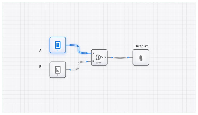
Explore the XNOR Simplified Circuit

Common Pitfall: Why Gray Code is Non-Negotiable

I often see students try to draw K-maps using standard binary ordering: 00, 01, 10, 11. It seems logical, right? Don’t do it.

If you use standard binary, you break the principle of adjacency. Look at the jump from 01 to 10. Both bits change ( $0 \to 1$ and $1 \to 0$ ). If you have ‘1’s in those two adjacent cells, you cannot simplify them because more than one variable is shifting. The Gray code sequence (00, 01, 11, 10) ensures that every single step you take on the map represents a change in exactly one variable. This is the “magic” that allows the math to work visually. Without Gray code, the K-map is just a confusing table; with it, it’s a calculator.

Verification with OSCILLOSCOPE_8CH

One of the most satisfying moments in digital engineering is proving that your “small” circuit does the exact same thing as the “big” one. On digisim.io, you can do this in real-time.

Build the Brute Force: Use eight AND gates and one massive OR gate to represent the original minterms.
Build the Optimized: Place a single XNOR gate (or the two-AND-one-OR equivalent) below it.
Sync the Inputs: Connect the same four INPUT_SWITCH components to both circuits.
Analyze: Connect the output of the brute-force circuit to Channel 1 of an OSCILLOSCOPE_8CH and the optimized output to Channel 2.

As you toggle the switches through all 16 combinations, the waveforms on the OSCILLOSCOPE_8CH will be identical. However, if you were to look at the propagation delay ( $t_{pd}$ ), you’d notice the optimized circuit responds significantly faster. In a high-speed CPU project, those nanoseconds are the difference between a 1MHz clock and a 10MHz clock.

Real-World Applications: Beyond the Classroom

K-maps aren’t just for passing exams; they are the bread and butter of hardware description.

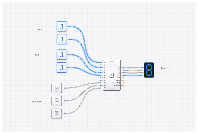
1. ALU Control Logic

In a typical 8-bit CPU, the ALU (Arithmetic Logic Unit) needs to know whether to add, subtract, or perform a bitwise AND based on an “opcode.” This opcode might be 4 bits wide. Engineers use K-maps to design the decoder logic that takes that 4-bit opcode and activates the specific control lines for the ADDER_8BIT or the COMPARATOR_8BIT. By minimizing this logic, they reduce the “instruction decode” time, which is a critical bottleneck in CPU performance.

2. Finite State Machines (FSMs)

Whether it’s a traffic light controller or a complex protocol handler, FSMs rely on “next-state logic.” This logic looks at the current state (stored in a REGISTER) and the current inputs to decide what the next state should be. These truth tables get massive quickly. K-maps allow designers to find the most efficient way to route those signals, often saving dozens of gates in the final implementation.

ALU Component Diagram

Common Pitfalls and “The Pro-Tip”

Even seasoned pros make mistakes. Here are the common mistakes I tell my students to watch out for:

Floating Inputs: When building your verification circuit on digisim.io, ensure every input of your AND gates is tied to something. A floating input in a simulator might behave predictably, but in a real circuit, it’s a recipe for chaos.
Missing the Wrap-Around: Always check the corners and the edges. Some of the most elegant simplifications come from grouping the four corners or the top and bottom rows.
Redundant Groups: Once all ‘1’s are covered, stop. Adding an extra group because “it looks nice” actually adds unnecessary gates to your circuit, defeating the purpose of the K-map.

The Power of Don’t Care Conditions

In many real designs, certain input combinations can never occur. For example, a BCD (Binary-Coded Decimal) system uses 4 bits to represent digits 0-9, so the combinations 1010 through 1111 never appear. In a K-map, you mark these impossible inputs with an $X$ (don’t care) instead of 0 or 1.

The key: you can treat each $X$ as either 0 or 1 — whichever helps you form a larger group. Since these inputs never occur in practice, it does not matter what the circuit outputs for them.

Example: Suppose a 4-variable function has 1s at cells 0, 2, 8, 10 and don’t cares at cells 1 and 3. Without the don’t cares, the four 1s (corners) group into $\overline{B}\overline{D}$ . But by treating cells 1 and 3 as 1s, you can form a larger group of 4 in the top row ( $\overline{A}\overline{B}$ ) plus the original corner group, potentially yielding a simpler total expression. Don’t care conditions frequently reduce the final gate count by 20-30% in real designs.

Take the Next Step in Your Curriculum

If you’re following our structured learning path on digisim.io, this deep dive bridges the gap between the basics of gates and the complexity of system design:

Boolean Algebra Fundamentals
Introduction to K-Maps (3-Variable)
Advanced K-Maps and Don’t Care Conditions
Designing a Custom ALU

The Karnaugh map turns a complex algebraic task into a visual puzzle. For functions of up to 4 variables, it reliably produces minimal SOP (or POS) expressions that Boolean algebra alone might miss. For functions of 5 or 6 variables, K-maps are still usable but become unwieldy; at that point, algorithmic methods like the Quine-McCluskey algorithm take over.

Ready to see the difference for yourself? Open the digisim.io editor, build the brute-force and optimized circuits from our example, and watch those waveforms align on the oscilloscope.

Start Building Your Optimized Circuit